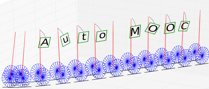
AutoMOOC
4th edition
Automation MOOC, Linear Control with a State Space approach
Open
Until
Luc Jaulin

Lab-STICC UBO GDR MACS GDR Robotique ENSTA Bretagne DGA ROBEX Sperob SAGIP


  1. Introduction
  2. Program with dates and points
  3. Post your work
  4. Files
  5. Lessons and Videos
  6. Other MOOCs
  7. Liste of students who got the diploma


Introduction

About AutoMOOC

AutoMOOC is a free course in English open to anyone. It corresponds to the book "Automation for robotics, Luc Jaulin (2015), ISTE editions" (see below).
To follow this course, you need to have some basics in mathematics (e.g., those that are required to enter an engineer school).


Registration

To register fill the form :
The registration is not mandatory to follow the MOOC and to see the videos. But it is needed to have to get the diploma.


Required

To follow AutoMOOC, you should have some basic notions in Python and knowledge in mathematics.
If you do not know Python, but any other programming language, you may learn easily the required notions in this MOOC.
You will have to install Python 3 in your machine.


Videos

A video with explanations related to each exercise is given as soon as the lesson opens. You are not obliged to follow the method that is given in the video.


Diploma

To get the diploma, you need at least 50 points. Therefore, doing all exercises is not mandatory.
The participants who got enough points will receive a diploma corresponding this MOOC.
This diploma can be used by students to obtain the corresponding ECTS from their PhD courses, or to comply with any other requests by their home university.
An example of the diploma you can obtain :


Program with dates and points

Lesson 1. Introduction , 12:00.
Exercise 1.1 Underwater robot (1 point)
Exercise 1.2 Sailboat robot (1 point)
Exercise 1.3 Chaotic system (1 point)
Exercise 1.4 Hénon Map (1 point)

Lesson 2. Lesson 2. Modeling , 12:00.
Exercise 2.1. First and second order systems (1 point)
Exercise 2.2. Mass-spring system (1 point)
Exercise 2.3. Model a pendulum (1 point)
Exercise 2.4. Hamilton method (1 point)
Exercise 2.5. Model an inverted rod pendulum (1 point)
Exercise 2.6. Model the Segway (1 point)
Exercise 2.7. Model a car (1 point)
Exercise 2.8. RLC circuit (1 point)
Exercise 2.9. DC-motor (1 point)
Exercise 2.10. Water tanks (1 point)
Exercise 2.11. Fibonacci sequence (1 point)
Exercise 2.12. Buses (1 point)

Lesson 3. Simulation , 12:00.
Exercise 3.1. Predator-prey model (1 point)
Exercise 3.2. Simple pendulum (1 point)
Exercise 3.3. Van der Pol (1 point)
Exercise 3.4. Simulation of a car (1 point)
Exercise 3.5. Integration with Taylor (1 point)
Exercise 3.6. Rotating cube (1 point)
Exercise 3.7. Three-dimensional simulation of a tricycle (1 point)
Exercise 3.8. Manipulator robot (1 point)
Exercise 3.9. Omni wheel robot (1 point)
Exercise 3.10. Snake (1 point)
Exercise 3.11. Swimbox (1 point)
Exercise 3.12. Virus (1 point)

Lesson 4. Linear systems , 12:00.
Exercise 4.1. Solution of a state equation (1 point)
Exercise 4.2. Stability criterion (1 point)
Exercise 4.3. Laplace variable (1 point)
Exercise 4.4. Transfer function of elementary systems (1 point)
Exercise 4.5. Transfer function of composite systems (1 point)
Exercise 4.6. Transfer matrix (1 point)
Exercise 4.7. Change of basis (1 point)
Exercise 4.8. Controllable canonical form (1 point)
Exercise 4.9. Second order system (1 point)
Exercise 4.10. Combination of systems (1 point)
Exercise 4.11. Transfer function (1 point)
Exercise 4.12. Canonical control form (1 point)
Exercise 4.13. Canonical observation form (1 point)
Exercise 4.14. Modal form (1 point)
Exercise 4.15. Jordan form (1 point)

Lesson 5. Linear control , 12:00.
Exercise 5.1. Non-observable states, non-controllable state (1 point)
Exercise 5.2. Using the controllability and observability criteria (1 point)
Exercise 5.3. Controllability criterion in discrete time (1 point)
Exercise 5.4. Controllability criterion in continuous time (1 point)
Exercise 5.5. Observability criterion (1 point)
Exercise 5.6. Kalman decomposition (1 point)
Exercise 5.7. Resolution of the pole placement equation (1 point)
Exercise 5.8. Output feedback of a scalar system (1 point)
Exercise 5.9. Separation principle (1 point)
Exercise 5.10. Proportional and derivative control of a pump (1 point)
Exercise 5.11. PID control (1 point)
Exercise 5.12. Canonical control form (1 point)
Exercise 5.13. State feedback with integral effect, monovariate case (1 point)
Exercise 5.14. State feedback with integral effect, general case (1 point)
Exercise 5.15. Luenberger observer (1 point)
Exercise 5.16. Demodulator (1 point)
Exercise 5.17. Output feedback of a non-strictly proper system (1 point)
Exercise 5.18. Output feedback with integral effect (1 point)
Exercise 5.19. Poincaré map (2 points)

Lesson 6. Linearized control , 12:00.
Exercise 6.1. Linearization of the predator-prey model (1 point)
Exercise 6.2. Water car (1 point)
Exercise 6.3. First order nonlinear system (1 point)
Exercise 6.4. State feedback (1 point)
Exercise 6.5. Control of the segway (2 points)
Exercise 6.6. Controlling an inverted rod pendulum (2 points)
Exercise 6.7. Linear Quadratic Regulator (1 point)
Exercise 6.8. Autonomous car (2 points)
Exercise 6.9. Follow the car (1 point)

All exercises should be posted: , 12:00.

Diplomas are sent by email: , 12:00.


Post your work

For each lesson, you should send your solution by email to jaulin.automooc@gmail.com
For the exercises that require the execution of a program, You should provide the Python (or other) code.
You should also send me a pdf file with some explanations and screen captures of the running program.
For some exercises, the solution corresponds to text and equations and no program is required. In such a case, you should post a scan of your paper sheet, (taken with you phone for instance) or any pdf file.


Files

Lessons and exercises in pdf.
Source code Latex + figures

Python start programs.
Librairy to be used autolib.py.


Lessons and videos


Lesson 1. Introduction

Open: Officially starts .
Lesson 1 is open in advance, to allow some adaptations and see how the MOOC works.

Abstract. Biological, economic or mechanical systems surrounding us can often be described by a state equations. This lesson introduces the notion of state, trajectory, inputs and outputs. It also presents the concepts of controller and closed-loop representation.


Exercise 1.1. Underwater robot
Exercise 1.2. Sailboat robot
Exercise 1.3. Chaotic system
Exercise 1.4. Hénon Map


View more : Effet papillon


Lesson 2. Modeling

Open:

Abstract. We will call modelling the procedure which consists of finding a more or less accurate state representation of the system we are looking at. In general, constant parameters appear in the state equations (such as the mass or the inertial moment of a body, the coefficient of viscous friction, the capacitance of a capacitor, etc.). In these cases, an identification step may prove to be necessary. Here, we will assume that all the parameters are known. Of course, no systematic methodology exists that can be used to model a system. The goal of this lesson and of the following exercises is to present, using several varied examples, how to obtain a state representation.


Exercise 2.1. First and second order systems

Exercise 2.2. Mass-spring system

Exercise 2.3. Model a pendulum

Exercise 2.4. Hamilton method

Exercise 2.5. Dynamic modeling of an inverted rod pendulum

Exercise 2.6. Dynamic modeling of the Segway

Exercise 2.7. Model a car

Exercise 2.8. RLC circuit

Exercise 2.9. DC-motor

Exercise 2.10. Water tanks

Exercise 2.11. Fibonacci sequence

Exercise 2.12. Buses


Lesson 3. Simulation

Open:

Abstract. In this chapter, we will show how to perform a computer simulation of a non-linear system described by its state equations. This step is important in order to test the behavior of a system (controlled or not). Before presenting the simulation method, we will introduce the concept of vector fields. This concept will allow us to better understand the simulation method as well as certain behaviors which could appear in non-linear systems. We will also give several concepts of graphics necessary for the graphical representation of our systems.


Exercise 3.1. Predator-prey model

Exercise 3.2. Simple pendulum
Start from the file pendumum.py.

Exercise 3.3. Van der Pol

Exercise 3.4. Simulation of a car

Exercise 3.5. Integration with Taylor
Start from the file taylor.py.

Exercise 3.6. Rotating cube

Exercise 3.7. Three-dimensional simulation of a tricycle

Exercise 3.8. Manipulator robot

Exercise 3.9. Omni wheel robot
Start from the file omniwheel.py.

Exercise 3.10. Snake
Start from the file snake.py.

Exercise 3.11. Swimbox

Exercise 3.12. Virus


Lesson 4. Linear systems

Open:

Abstract. The study of linear systems is fundamental for the proper understanding of the concepts of stability and the design of linear controllers. This lesson introduces the notion of stability and makes the link between a state space representation and the more classical transfer approach.


Exercise 4.1. Solution of a state equation

Exercise 4.2. Stability criterion

Exercise 4.3. Laplace variable

Exercise 4.4. Transfer function of elementary systems

Exercise 4.5. Transfer function of composite systems

Exercise 4.6. Transfer matrix

Exercise 4.7. Change of basis

Exercise 4.8. Controllable canonical form

Exercise 4.9. Second order system

Exercise 4.10. Combination of systems

Exercise 4.11. Transfer function

Exercise 4.12. Canonical control form

Exercise 4.13. Canonical observation form

Exercise 4.14. Modal form

Exercise 4.15. Jordan form


Lesson 5. Linear control

Open:

Abstract. We will study the design of controllers for systems given by linear state equations. After having defined the fundamental concepts of controllability and observability, we will propose two approaches for the design of controllers. First of all, we will assume that the state is accessible on demand. Even though this hypothesis is generally not verified, it will allow us to establish the principles of the pole placement method. In the second phase, we will no longer assume that the state is accessible. We will then have to develop state estimators capable of approximating the state vector in order to be able to employ the tools developed in the first phase.


Exercise 5.1. Non-observable states, non-controllable state

Exercise 5.2. Using the controllability and observability criteria

Exercise 5.3. Controllability criterion in discrete time

Exercise 5.4. Controllability criterion in continuous time

Exercise 5.5. Observability criterion

Exercise 5.6. Kalman decomposition

Exercise 5.7. Resolution of the pole placement equation

Exercise 5.8. Output feedback of a scalar system

Exercise 5.9. Separation principle

Exercise 5.10. Proportional and derivative control of a pump

Exercise 5.11. PID control

Exercise 5.12. Canonical control form

Exercise 5.13. State feedback with integral effect, monovariate case

Exercise 5.14. State feedback with integral effect, general case

Exercise 5.15. Luenberger observer

Exercise 5.16. Demodulator

Exercise 5.17. Output feedback of a non-strictly proper system

Exercise 5.18. Output feedback with integral effect

Exercise 5.19. Poincaré map


Lesson 6. Linearized control

Open:

Abstract. In the previous chapter, we have shown how to design controllers for linear systems. However, in practice, the systems are rarely linear. Nevertheless, if their state vector remains localized in a small zone of the state space, the system may be considered linear and the linear techniques can then be used. We will first show how to linearize a non-linear system around a given point of the state space. We will then discuss how to stabilize these non-linear systems.


Exercise 6.1. Linearization of the predator-prey model

Exercise 6.2. Water car

Exercise 6.3. First order nonlinear system

Exercise 6.4. State feedback

Exercise 6.5. Control of the segway
Start from the files segway.py and segway3D.py

Exercise 6.6. Controlling an inverted rod pendulum
Start from the file invpend.py.

Exercise 6.7. Linear Quadratic Regulator
Start from the file lqr.py.

Exercise 6.8. Autonomous car
Start from the file circuit.py.

Exercise 6.9. Follow the car


List of the students who got the diploma

Matias Barla
Evandro Bernardes
Jules Lesaulnier
Paul Pineau
Agustin Zorzano
Emmanuel Charron
Jean-Louis Cougnon
Bastien Depeyre
Isabelle Maroger
Steven Wang
Théo Chassanite
Stéphane Yang
Ahmad Hably
Wanchen Li
Dimitri Léca
Ronan Guermeur
Georges Daher
Jose Eduardo Carvajal Rubio
Bernardo Hummes Flores
Camille Apamon
Marwan Johra
Mathilde Roques
Célia Saghour
Sylvain Hernandez
Amine Lagzouli
Abdelhaq Ouelli
Michele Grimaldi
Abdelrahman Sayed Ibrahim
Hugo Rémin
Julien Brisset