Rolling

Proving the stability of the rolling navigation

Acta Cybernetica

Here are given the Python programs associated with the paper. You can also execute them directly using replit.com.

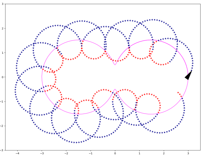
Simulation of the rolling

Python program illustrating the rolling along the Hippopède de Proclus.
You can directly run it with replit.com

The corresponding code can also be found below.

from roblib import *
def clock_control(x,q,c):     x1,x2,ψ=x.flatten()
    U = {0:1, 1:2}
    c=c+dt
    φ=a**2*x1**2+b*b*x2**2-(x1**2+x2**2)**2
    if (q==0)&(φ>0)&(c>1) :
       q=1
       c=-pi/2
    if (q==1)&(c>0): q=0
    col = {0:'darkblue', 1:'red'}
    pause(0.001)
    draw_tank(x,col[q],0.01,1)
    u=U[q]
    return q,c,u

def clock_robot(x,u):
    x1,x2,ψ=x.flatten()
    x=x+dt*array([[cos(ψ)], [sin(ψ)],[u]])
    return x

a,b=3,0.5
x=array([[a],[0],[1]])
ax=init_figure(-4.5,3.5,-3,3)
T=arange(0,7,0.01) #Hippopède de Proclus
plot(a*b*b*cos(T)/(b*b*cos(T)**2+a*a*sin(T)**2),a*a*b*sin(T)/(b*b*cos(T)**2+a*a*sin(T)**2),'magenta', linewidth = 1)
q,c=0,0
dt=0.1
for t in arange(0,70,dt):
    q,c,u=clock_control(x,q,c)
    x=clock_robot(x,u)

Simulation of the rolling in the 3d state space

Python program illustrating the role of the Poincaré sections.
You can directly run it with replit.com

from roblib import *
def clock_control(x,q,c):
    x1,x2,ψ=x.flatten()
    U = {0:1, 1:2}
    c=c+dt
    φ=-x2
    if (q==0)&(φ>0)&(c>1) : q=1; c=-pi/2; ψ=ψ-2*pi
    if (q==1)&(c>0): q=0; c=0
    col3d= {0:'green',1:'blue'}
    shad= {0:'gray',1:'black'}
    ax.scatter(c,x2,ψ,color=col3d[q],s=1)
    ax.scatter(c,x2,-s,color=shad[q],s=1)
    ax.scatter(c,s,ψ,color=shad[q],s=1)
    ax.scatter(s,x2,ψ,color=shad[q],s=1)
    pause(0.001)
    u=U[q]
    x=array([[x1],[x2],[ψ]])
    return x,q,c,u

def clock_robot(x,u,dt):
    x1,x2,ψ=x.flatten()
    x=x+dt*array([[cos(ψ)], [sin(ψ)],[u]])
    return x

fig = figure()
ax = Axes3D(fig)
s=5
clean3D(ax,-5,5,-5,5,-5,5)
draw_axis3D(ax,0,0,0,eye(3))
size=1
S0=tran3H(0,0,pi/2)@diag([0.01,size,size,1]) @ tran3H(-0.5,-0.5,-0.5)@cube3H()
draw3H(ax, S0, 'red', False)
S1=tran3H(pi,0,3*pi/2)@diag([size,0.01,size,1]) @ tran3H(-0.5,-0.5,-0.5)@cube3H()
draw3H(ax, S1, 'red', False)
S2=tran3H(-pi/2,0,-pi/2)@diag([size,0.01,size,1]) @ tran3H(-0.5,-0.5,-0.5)@cube3H()
draw3H(ax, S2, 'red', False)

x=array([[2],[0],[pi/2]])
q,c=0,0
dt=0.03
for t in arange(0,3*pi/2,dt):
    q_=q
    x,q,c,u=clock_control(x,q,c,dt)
    x=clock_robot(x,u,dt)

The first bassin

We propose a Python program able to find the first bassin with is the box X0=[-0.1, 0.1]x[-0.1, 0.1]. For each point initiated in X0, we converge to x=0
You can directly run it with replit.com

from codac import *
x2=Interval(-0.1,0.1)
x3=Interval(-0.1,0.1)
A=sqrt(1-(x2-sin(x3))**2)
J=IntervalMatrix(2,2)
J[0][0]=Interval(1,1)
J[0][1]=-cos(x3)
J[1][0]=1/A
J[1][1]=-cos(x3)/A
X=IntervalVector(2)
X[0]=x2
X[1]=x3
print('\nJ=',J)
print('\nX=',X)
print('\nJ*X=',J*X)
print('\n(J*J)*X=',(J*J)*X)

Characterization of the attraction bassin

Python program illustrating the characterization of an attraction bassin
You can directly run it with replit.com

from codac import *
from vibes import *
X0=IntervalVector([[-1.1, 1.1], [-1.1, 1.1]])
p1 = Function("x2", "x3","(x2-sin(x3);asin(x2-sin(x3)))")
p2 = Function("x2", "x3","(0 ; 0)")
f_dom1= Function("x2", "x3", "x2-sin(x3)")
f_box = Function("x1","x2","(x1,x2)")
S0 = SepFwdBwd(f_box, IntervalVector([[-0.1, 0.1],[-0.1, 0.1]]))
S1 = SepFwdBwd(f_dom1, Interval(-3.14/2,3.14/2)) & SepInverse(S0, p1)
S2 = SepFwdBwd(f_dom1, Interval(-3.14/2,3.14/2)) & SepInverse(S0, p2)
vibes.beginDrawing()
vibes.newFigure('rolling')
vibes.setFigureSize(1000,1000)
params = {'color_in': 'black[green]', 'color_out':'black[blue]', 'color_maybe':'white[white]'}
pySIVIA(X0,S2,0.01,draw_boxes=True, **params)
params = {'color_in': 'black[orange]', 'color_out':'transparent[transparent]', 'color_maybe':'white[white]'}
pySIVIA(X0,S1,0.01,draw_boxes=True, **params)
params = {'color_in': 'black[red]', 'color_out':'transparent[transparent]', 'color_maybe':'white[white]'}
pySIVIA(X0,S0,0.01,draw_boxes=True, **params)
vibes.axisEqual()

Codac program to compute the Poincaré time

Python program illustrating how to compute the time at which we cross the surface.
You can directly run it with replit.com

from vibes import *
from codac import *
tmax=4
dx=0.1
T = Interval(0,tmax)
dt = 0.001
x = TubeVector(T, dt, tmax)
x0 = IntervalVector([[0,0], [-dx, dx],[3.1416/2-dx,3.1416/2+dx]])
x.set(x0, 0.)
f = Function("x1", "x2","x3", "(1;sin(x3);1)")
ctc_f = CtcLohner(f)
ctc_f.contract(x)
g2=x[1]
dg2=sin(x[2])
#c=max(g2,dg2)
ctc_max = CtcFunction(Function("x1", "x2","x3", "max(x1,x2)-x3"), Interval(0,0))
M= TubeVector(T, dt, tmax)
M[0]=g2
M[1]=dg2
ctc_max.contract(M)
c=M[2]
beginDrawing()
fig.set_properties(50, 50, 800, 800)
fig.axis_limits(IntervalVector([[0, tmax], [-2, 2]]))
fig.add_tube(g2, 'g2',"blue[lightGray]")
fig.add_tube(dg2, 'dg2',"blue[magenta]")
fig.add_tube(c, 'c',"green[blue]")
ti=Interval(0,tmax)
yi = Interval(-0.01,0.01)
ctc_eval = CtcEval()
ctc_eval.contract(ti, yi, c)

C++ code for the proof of stability using CAPD library

#include
#include "capd/capdlib.h"
using namespace capd;
using namespace capd::autodiff;
using namespace std;
int main(int argc, char * argv[])
{
// System
const int dim = 3, order = 5, nbParams = 1;
double initTime = 0;
// Initial condition
IVector a = {{-.01, .01}, {-.01, .01}};
IVector x = {{0., 0.}, a[0], a[1] + M_PI_2};
// Doubleton representing initial condition
C1Rect2Set set(x, initTime);
// define vector field
std::function f = [](
Node, Node in[], int,
Node out[], int, Node params[], int) {
out[0] = Node(1);
out[1] = sin(in[2]);
out[2] = params[0];
};
IMap vf(f, dim, dim, nbParams);
vf.setParameter(0, 1.);

// define solver
IOdeSolver solver(vf, order);

// poincare time
interval tau;
// monodromy matrix
IMatrix monodromyMatrix(3, 3);

// define section
ICoordinateSection section_1(dim, 0, 0.); // x1 = 0.
ICoordinateSection section_2(dim, 1, 0.); // x2 = 0.
// define poincare map
IPoincareMap poincare_map(solver, section_2, poincare::PlusMinus);

// define chart matrices
IMatrix H2 = {{1, 0, 0}, {0, 0, 1}};
IMatrix H1 = {{0, 0}, {1, 0}, {0, 1}};
IMatrix H1_T = {{0, 1, 0}, {0, 0, 1}};
IMatrix H2_T = {{1, 0}, {0, 0}, {0, 1}};
IMatrix Jp_1_2 = {{0, 0}, {0, 1}};

/*************************
* FIRST ITERATION
*************************/

// evaluate poincare map to get x and tau
x = poincare_map(set, monodromyMatrix, tau);
// evaluate Jacobian of poincare map
IMatrix Jq = poincare_map.computeDP(x, monodromyMatrix, tau);
IMatrix Jp_0 = H2 * Jq * H1;

cout << "tau_b : " << tau << endl
<< "x_b : " << x << endl
<< "Jq : " << Jq << endl
<< "monodromy : " << monodromyMatrix << endl
<< "Jp_0 : " << Jp_0 << endl
<< endl;
// tau_b : [3.1114,3.17179]
// x_b : {[3.1114,3.17179],[-0.0603952,0.0603829],[4.67219,4.75259]}
// Jq : {
// {[1,1],[1,1.00081],[-2.02159,-1.97913]},
// {[-4.00162e-300,4.00162e-300],[-0.000808656,0.000808002],[-0.0424262,0.0424605]},
// {[-4.00162e-300,4.00162e-300],[1,1.00081],[-1.02159,-0.979133]}
// }
// monodromy : {
// {[1,1],[-2e-300,2e-300],[-6.03992e-300,6.03992e-300]},
// {[-2e-300,2e-300],[1,1],[-2.01996,-1.97913]},
// {[-2e-300,2e-300],[-2e-300,2e-300],[1,1]}
// }
// Jp_0 : {
// {[1,1.00081],[-2.02159,-1.97913]},
// {[1,1.00081],[-1.02159,-0.979133]}
// }

// reinitialize clock and heading
x = {{-M_PI_2, -M_PI_2}, {0., 0.}, x[2] - 2 * M_PI};
set = C1Rect2Set(x, initTime);
// change vector field parameter
vf.setParameter(0, 2.);
// define new section
poincare_map.setSection(section_1);
poincare_map.setCrossingDirection(poincare::MinusPlus);

// evaluate poincare map to get x and tau
x = poincare_map(set, monodromyMatrix, tau);
// evaluate Jacobian of poincare map
Jq = poincare_map.computeDP(x, monodromyMatrix, tau);
IMatrix Jp_1 = H1_T * Jq * H2_T;

cout << "tau_b : " << tau << endl
<< "x_b : " << x << endl
<< "Jq : " << Jq << endl
<< "monodromy : " << monodromyMatrix << endl
<< "Jp_1 : " << Jp_1 << endl
// tau_b : [1.5708,1.5708]
<< endl;
// x_b : {[0,0],[-0.0417802,0.0417865],[1.5306,1.611]}
// Jq : {
// {[-0,0],[0,0],[0,0]},
// {[-1,-0.999192],[1,1],[0.958986,1.03941]},
// {[-2,-2],[0,0],[1,1]}
// }
// monodromy : {
// {[1,1],[0,0],[0,0]},
// {[-1.12193e-318,1.12193e-318],[1,1],[0.958986,1.03941]},
// {[0,0],[0,0],[1,1]}
// }
// Jp_1 : {
// {[-1,-0.999192],[0.958986,1.03941]},
// {[-2,-2],[1,1]}
// }

// applying centred form algorithm
auto p_a = Jp_1 * Jp_1_2 * Jp_0 * a;
x = {0, p_a[0], p_a[1] + M_PI_2};

cout << "p_a : " << p_a << endl << endl;
// p_a : {[-0.021021,0.021021],[-0.020224,0.020224]}

/*************************
* SECOND ITERATION
*************************/

set = C1Rect2Set(x, initTime);
// change vector field parameter
vf.setParameter(0, 1.);
// define new section
poincare_map.setSection(section_2);
poincare_map.setCrossingDirection(poincare::PlusMinus);

// evaluate poincare map to get x and tau
x = poincare_map(set, monodromyMatrix, tau);
// evaluate Jacobian of poincare map
Jq = poincare_map.computeDP(x, monodromyMatrix, tau);
IMatrix Jp_0_bis = H2 * Jq * H1;

cout << "tau_b : " << tau << endl
<< "x_b : " << x << endl
<< "Jq : " << Jq << endl
<< "monodromy : " << monodromyMatrix << endl
<< "Jp_0_bis : " << Jp_0_bis << endl
<< endl;
// tau_b : [3.07934,3.2039]
// x_b : {[3.07934,3.2039],[-0.124531,0.124429],[4.62991,4.79492]}
// Jq : {
// {[1,1],[1,1.00342],[-2.04723,-1.95593]},
// {[-4.00683e-300,4.00683e-300],[-0.00341529,0.00340366],[-0.0909928,0.0913036]},
// {[-4.00683e-300,4.00683e-300],[1,1.00342],[-1.04723,-0.955927]}
// }
// monodromy : {
// {[1,1],[-2e-300,2e-300],[-6.08053e-300,6.08053e-300]},
// {[-2e-300,2e-300],[1,1],[-2.04026,-1.95593]},
// {[-2e-300,2e-300],[-2e-300,2e-300],[1,1]}
// }
// Jp_0_bis : {
// {[1,1.00342],[-2.04723,-1.95593]},
// {[1,1.00342],[-1.04723,-0.955927]}
// }

// reinitialize clock and heading
x = {{-M_PI_2, -M_PI_2}, {0., 0.}, x[2] - 2 * M_PI};
set = C1Rect2Set(x, initTime);
// change vector field parameter
vf.setParameter(0, 2.);
// define new section
poincare_map.setSection(section_1);
poincare_map.setCrossingDirection(poincare::MinusPlus);

// evaluate poincare map to get x and tau
x = poincare_map(set, monodromyMatrix, tau);
// evaluate Jacobian of poincare map
Jq = poincare_map.computeDP(x, monodromyMatrix, tau);
IMatrix Jp_1_bis = H1_T * Jq * H2_T;

cout << "tau_b : " << tau << endl
<< "x_b : " << x << endl
<< "Jq : " << Jq << endl
<< "monodromy : " << monodromyMatrix << endl
<< "Jp_1_bis : " << Jp_1_bis << endl
<< endl;
// tau_b : [1.5708,1.5708]
// x_b : {[0,0],[-0.0890083,0.0890592],[1.48832,1.65333]}
// Jq : {
// {[-0,0],[0,0],[0,0]},
// {[-1,-0.996596],[1,1],[0.914151,1.07914]},
// {[-2,-2],[0,0],[1,1]}
// }
// monodromy : {
// {[1,1],[0,0],[0,0]},
// {[-1.13804e-318,1.13804e-318],[1,1],[0.914151,1.07914]},
// {[0,0],[0,0],[1,1]}
// }
// Jp_1_bis : {
// {[-1,-0.996596],[0.914151,1.07914]},
// {[-2,-2],[1,1]}
// }

auto p_p_a = Jp_1_bis * Jp_1_2 * Jp_0_bis * Jp_1 * Jp_1_2 * Jp_0 * a;

cout << "p_p_a : " << p_p_a << endl;
cout << "p_p_a is " << ((a[0].contains(p_p_a[0]) and a[1].contains(p_p_a[1])) ? "in " : "not " "in ") << "a" << endl;
// p_p_a : {[-0.00512577,0.00512577],[-0.00178467,0.00178467]}
// p_p_a is in a

return EXIT_SUCCESS;
}